Land Surface Temperature Anomalies as Indicators of Urban Land Cover Change—A Study of Two Indian Cities

Introduction

Urban areas are the engines of economic growth and the number of people living in urban areas is increasing continuously worldwide. Urban land cover is undergoing continuous transformation due to the increasing population and the need for better facilities. The development of new urban features such as buildings, roads, etc., often leads to the conversion of natural surfaces into non-evaporating, impervious surfaces, which affect the energy balance at the surface (Yuan and Bauer, 2006). As a result, the temperature in urban areas is higher than in peripheral suburban areas, and this phenomenon is known as the urban heat island (UHI) effect (Chen et al., 2023). Changes in land use and land cover (LULC) during the process of urbanisation play a significant role in determining the spatial distribution of land surface temperature (LST). This has been demonstrated in real-world examples, such as the expansion of buildings and roads and the reduction of water bodies, trees, and agricultural land. These observations support the notion that LULC changes are responsible for the UHI effect (Zhao et al., 2017). The thermal characteristics of the urban surface materials and the lack of surface evaporation increase the outgoing longwave radiation resulting in increased LST over urban areas (Dousset and Luvall, 2019; Li et al., 2019). This increased LST over urban areas compared to the surrounding rural areas is commonly known as the Surface Urban Heat Island (SUHI) effect and can be detected using thermal infrared sensors aboard various satellites (Deilami et al., 2018; Zhou et al., 2018). Traditionally, SUHI is defined as the difference in LST observed over urban and rural areas (Shastri and Ghosh, 2019), which suggests that the SUHI intensity (SUHII) also depends on the surface conditions of the pixels classified as rural in the analysis. Although SUHII is a useful indicator of urbanisation, it may not help in planning urban heat mitigation measures in different parts of a city (Martilli et al., 2020). In many developing countries, urban development often takes place in an unplanned manner leading to a lack of proper information for the city planning authority. For better planning, city planners need to understand how a given area’s thermal conditions change over time and relative to other areas of a city. Understanding how LST are structured across the urban landscape can help enhance sustainability. Landscape changes from vegetation to the built environment associated with urbanisation processes have been linked to an increase in urban LST (Stewart and Kremer, 2022). Multi-temporal land cover maps are widely used to identify spatiotemporal changes in urban land cover. However, manually inferring thermal conditions from land cover maps is difficult. Furthermore, errors in each land cover map can be compounded, leading to reduced accuracy of the land cover change map (Zhu, 2017). Keith et al. (2019) mentioned that planners find it challenging to infer details from satellite images and a more direct representation of the thermal conditions of a city is needed to aid planners. Therefore, it is necessary to clearly identify the spatiotemporal changes in the thermal characteristics of cities at a finer level. This becomes even more critical during the planning or evaluation phase of heat mitigation measures.

LST is one of the indicators used to examine the thermal heterogeneity of the Earth’s surface and the impact on surface temperatures of natural and human-induced changes (Mildrexler et al., 2018). Previous studies (Julien and Sobrino, 2008; Mildrexler et al., 2009; Sobrino and Raissouni, 2010) have combined LST with vegetation indices to map land cover changes with 1 km spatial resolution on annual time scales. Time series analysis of LST from the MODIS sensor has been used to identify changes in wetlands over Tanzania (Muro et al., 2018) and Mildrexler et al. (2018) demonstrated that anomalies in annual maximum LST could indicate regions affected by drought, heatwaves, forest loss and ice melt. The change in urban land cover will affect the normal LST conditions experienced over a given area, causing a change in the magnitude and/or direction of the LST anomaly. Therefore, LST anomalies can signal a change in land cover conditions and indicate whether an area is warmer or cooler. This study aims to test whether LST anomalies can identify changes in land cover and thermal conditions over urban areas. Focussing on changing thermal regimes has the potential to detect shifts in ecosystems towards thresholds of profound change (Grumm and Hart, 2001). LST data from Landsat thermal infrared (TIR) images acquired during summer (March, April and May) from 1988 to 2020 was used to estimate LST anomalies. LST is high in summer because impervious surfaces can increase the surface sensible heat flux, which in turn increases LST (Han et al., 2022). This study evaluates summer LST anomalies to understand extreme heat situations, thus paving the way to prepare a master plan for a resilient city that can adapt to heat stress. The information can be used to prioritise the allocation of resources for green infrastructure, such as parks and trees, in areas most susceptible to heat stress. It can help city planners make informed decisions about where to focus their efforts and resources as they develop their heat resilience master plans.

Study area and datasets

The Chennai Metropolitan area and the Navi Mumbai Municipal corporation area located in the Indian states of Tamil Nadu and Maharashtra respectively were selected for the study (Figure 1). Both of these coastal cities are unique urban centres because of the varying land cover/land use conditions and the rich biodiversity. In Chennai, the minimum air temperature varies between 17°C and 25°C and the maximum air temperature ranges from 30°C to 38°C. Over Navi Mumbai, the temperature is between 17°C and 20°C in the winter while the summer temperature ranges from 36°C to 41°C. The month of May generally records the annual maximum temperature in both cities. Navi Mumbai is bordered by mangroves on the west (creek side) and hills on the east side respectively. Similarly, Chennai has a biodiversity-rich national park and three rivers within the city. These natural elements play an important role in defining the local climate in both of these cities.

Figure 1. Study Area - (A) Chennai and (B) Navi Mumbai (Image source: Google Earth).

The majority of the previous studies to identify land cover change using LST have used MODIS or AVHRR data at 1 km resolution. However, over urban areas, this spatial resolution may not be sufficient to identify finer changes so data from the Landsat series of satellites acquired from 1988 to 2020 were used in the present study. Data acquired during March, April and May in each year were used for the analysis as this increased the chance of obtaining clear sky images and also coincided with the months when higher LST and air temperatures were observed. Thermal infrared radiance was obtained from the level-1 product and surface reflectance in the visible and near-infrared bands was obtained from the corresponding level-2 datasets.

We also used LULC maps for the years 1990, 2000, 2010, and 2017 over Navi Mumbai. The LULC maps were created with Landsat data at 30 m resolution using the Supervised Maximum Likelihood Classifier (SMLC). The SMLC assigns a pixel to a specific class based on its maximum possible occurrence in that class based on the training data. Mainly, five classes were classified including water bodies, mangroves, other vegetation, developed (i.e. built up) areas, and barren land. Although many advanced machine learning algorithms exist for land cover classification, the classic SMLC was used as its ability to produce relatively accurate land cover maps is well established. In addition, in this case, the land cover classification scheme had only five classes, which were easily distinguishable by the algorithm using the multispectral Landsat data. The training and validation data were obtained from Google Earth Engine (GEE). These LULC maps were used by Azeez et al. (2022) to identify mangrove areas over Navi Mumbai and in this study, we have used the LULC maps to identify the urban growth. The overall accuracy of the land cover maps was found to be more than 85% for all the years. Additional details about the creation of LULC maps and their accuracy assessment can be obtained from Azeez et al. (2022).

Methodology

The different steps followed in this study are described in this section. The entire analysis was performed on the GEE platform using Landsat images with a pixel size of 30 m.

Retrieval of LST

The LST required for the study was retrieved from Landsat level-1 product using the Statistical Mono Window Algorithm (SMWA), which is based on the empirical relationship between Top of the Atmosphere (TOA) brightness temperature in a single thermal band, land surface emissivity in the corresponding band and LST (Ermida et al., 2020). The surface emissivity required for the LST retrieval was obtained using a modified vegetation index (VI) based model (Kodimalar et al., 2020). The retrieved LST was not validated due to the lack of any in situ thermal radiometer data over the study areas. However, the models used for the retrieval of emissivity and LST were found to retrieve LST with accuracy better than that of the Landsat-level 2 surface temperature product (Harod et al., 2021) and hence were used in this study. LST values were estimated for all clear sky images in March, April and May and a 3-month average available LST was estimated for the two study regions. This 3-month average LST was used for further analysis.

LST Anomaly

We defined LST anomalies in both spatial and temporal domains. For the temporal LST anomaly, the long-term temporal mean (LST_mean) and standard deviation (LST_std) of LST from 1988 to 2020 were estimated for each pixel over the study area from all available valid LST values. Then, the standardised temporal LST anomaly (${\text{LST}}_{\text{ano}}^{\mathrm{T}}$) for each year (i) from 1988 to 2020 was calculated as given in Equation 1.

where LST [i] represents the 3-month average LST for each year. The ${\text{LST}}_{\text{ano}}^{\mathrm{T}}$ represents the number of standard deviations by which the anomaly deviates from the long-term normal, providing information on the relative significance of anomalous features and how they vary across different land cover types (Mildrexler et al., 2018). The time series of ${\text{LST}}_{\text{ano}}^{\mathrm{T}}$ was analysed on a pixel-by-pixel basis to identify the temporal changes associated with urbanisation.

The standardised spatial LST anomaly ($\left.{\text{LST}}_{\text{ano}}^{\mathrm{S}}\right)$ was defined as the deviation from the average LST conditions found within the respective urban boundary as given in Equation 2

where, ${\text{LST}}_{\text{mean}}^{\mathrm{S}}$ and ${\text{LST}}_{\text{std}}^{\mathrm{S}}$ represent the spatial mean and standard deviation of LST of all the pixels within the urban boundary for each year i. The spatial mean and standard deviation of LST were estimated from the 3-month (March, April and May) average LST estimated for each year. The spatial anomaly was defined based on the assumption that each city will have a mix of low temperature (e.g., vegetated surfaces and water bodies) and high temperature (e.g., dry barren land, paved surfaces) areas and the anomaly will be negative and positive respectively for these two types of surfaces. As a surface changes from its natural state to an impervious state, the anomaly will shift in magnitude and direction as a response to this change.

The temporal and spatial LST anomalies were then used to identify changes in urban surface temperature conditions on a 5-year basis starting with the year 1990 (e.g., changes between 1990 and 1995, 1995 and 2000, etc.). The time series of the LST anomaly was analysed within the given 5-year block on a pixel-by-pixel basis and if the anomaly was positive (negative) for 80% of the 5-year block then that particular pixel was labelled as a warm (cool) pixel. If the value fluctuated around zero, without being positive or negative for 80% of the time, then the pixel was categorised under the “cannot say” category. The 80% threshold was a strict criterion enforced to identify only pixels with a definite change over the 5 years and to further reduce false positives.

Estimation of SUHII

The spatial LST anomaly defined in this study is conceptually similar to surface urban heat island intensity (SUHII) and to understand the relationship between them SUHII maps were generated. For each 5-year block, the annual 3-month LST was averaged to define a 5-year average LST for March, April and May (LST₅). Using this 5-year average LST, the 5-year SUHII was defined as in Equation 3.

where LST_5v is the mean LST value estimated over urban vegetation such as parks and other natural vegetation. Vegetated areas within each city were identified by visible interpretation and a mean LST of these vegetated surfaces was considered LST_5v. SUHII was defined in this manner to know the temperature differences between different locations in the city and the vegetated areas within the city. This definition avoids the influence of rural areas surrounding the city and in addition, this definition is closer to the SUHII defined using the Local Climate Zone (LCZ) concept (Stewart and Oke, 2012; Bechtel et al., 2019; Geletič et al., 2019). The SUHII maps were developed with colour coding, where green represents cooler spots followed by yellow and then red shows the hotter spots in the city.

Results and Discussions

Temporal Anomaly

${\text{LST}}_{\text{ano}}^{\mathrm{T}}$ estimated each year was first visually analysed to understand its spatiotemporal variation and relationship with land cover. Examples of ${\text{LST}}_{\text{ano}}^{\mathrm{T}}$ are presented in Figure 2. Positive anomalies (${\text{LST}}_{\text{ano}}^{\mathrm{T}}>0$) indicate warmer conditions than the long-term mean, shown in yellow and reddish hues, and negative anomalies (${\text{LST}}_{\text{ano}}^{\mathrm{T}}<0$) indicate cooler conditions than the long-term average LST, shown in green and blue hues. Since the seasonally average LST varies every year, the ${\text{LST}}_{\text{ano}}^{\mathrm{T}}$ also exhibits temporal variations. In general, it was observed that when the land cover of the pixel changes from a natural condition to an impervious or developed state, the temporal LST anomaly changes its sign from negative to positive. An example of this is presented in Supplementary Figure S1.

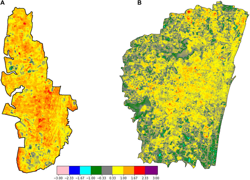
Figure 2. Examples of temporal LST anomaly observed over (A) Navi Mumbai for the year 2019 and (B) Chennai for the year 2020.

Figures 3, 4 show the thermal condition of a pixel over Navi Mumbai and Chennai respectively analysed on a 5-year basis. Both figures show that there has been a significant increase in the number of warmer pixels over both cities in recent years as compared to the past. In particular, the most recent 5-year block of 2015–2020 appears to be the warmest with a large number of pixels being categorised as warm. The warming pattern captured by the temporal LST anomalies may also be due to a positive trend in the LST. In both cities, over surfaces that changed from a natural state to other states (such as impervious urban surfaces), the temporal LST anomaly exhibited a clear change in sign from negative to positive and remained positive for many years after the change occurred. This observation aligns with previous studies highlighting the impact of urbanisation on LST. For instance, Zhao et al. (2014) demonstrated that urban expansion significantly increases surface temperatures due to the replacement of vegetated areas with heat-absorbing materials. Similarly, Li et al. (2017) found that urban areas consistently show higher LST than their rural counterparts, largely due to increased impervious surfaces and reduced vegetation. The temporal analysis also indicated that the period from 2015 to 2020 was the warmest in both cities, with a significant increase in the number of warmer pixels. This trend is consistent with global observations of rising urban temperatures due to climate change and urban sprawl. According to the Intergovernmental Panel on Climate Change (IPCC, 2021), urban areas are particularly vulnerable to heat waves and rising surface temperatures, which exacerbate the UHI effect.

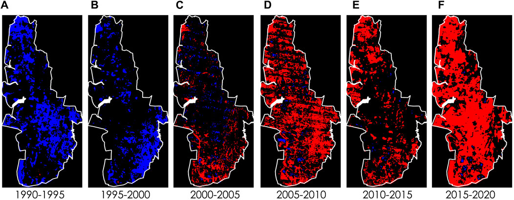
Figure 3. Thermal conditions of pixels identified from the temporal LST anomaly over Navi Mumbai. Red and blue colours indicate warmer and cooler pixels respectively. Black colour indicates that the pixel cannot be labelled as either warm or cool based on the adopted criteria. Each sub-plot from (A–F) indicates a 5-year block starting 1990.

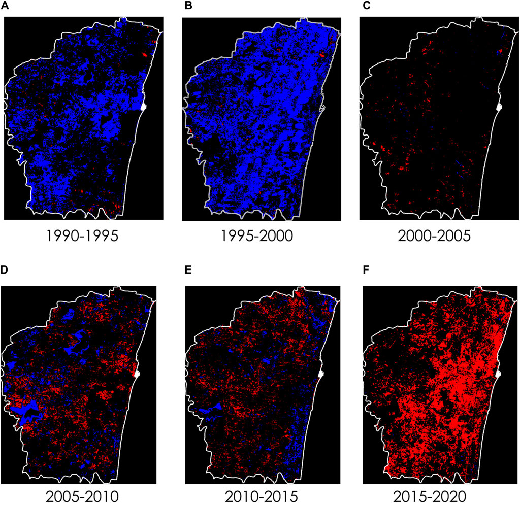
Figure 4. Thermal conditions of pixels identified from the temporal LST anomaly over the Chennai Metropolitan area. Red and blue colours indicate warmer and cooler pixels respectively. Black colour indicates that the pixel cannot be labelled as either warm or cool based on the adopted criteria. Each sub-plot from (A–F) indicates a 5-year block starting 1990.

Spatial Anomaly

While the temporal anomalies indicate the change in the LST of a particular pixel concerning its long-term mean, the spatial anomalies (${\text{LST}}_{\text{ano}}^{\mathrm{S}}$) will indicate the deviation in the LST of a pixel concerning the LST of vegetated areas within the urban boundary. Thus, the spatial LST anomaly will indicate how warm or cool a pixel is about the vegetated areas in the city. Examples of spatial LST anomalies estimated over Navi Mumbai in 2019 and over Chennai in 2020 are presented in Figure 5. From the ${\text{LST}}_{\text{ano}}^{\mathrm{S}}$ maps, it is clearly observed that water bodies and vegetated surfaces have negative anomalies while developed and other impervious surfaces have positive anomalies.

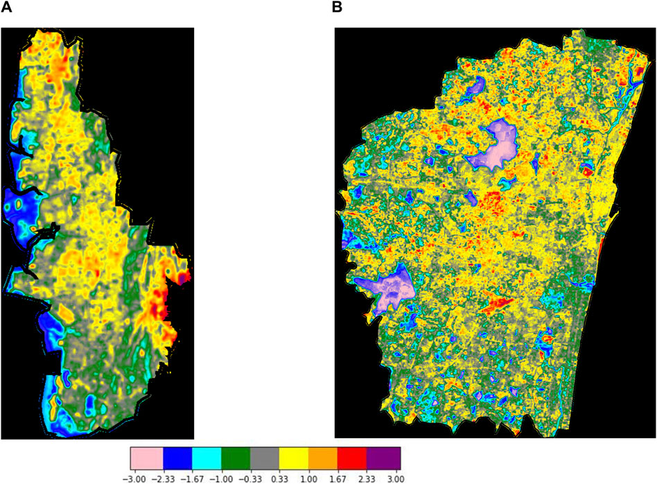
Figure 5. Examples of spatial LST anomaly observed over (A) Navi Mumbai for the year 2019 and (B) Chennai for the year 2020.

Similarly, with the spatial LST anomalies, we labelled each pixel as warm, cool and “cannot say” classes using the same 80% threshold criteria in each 5-year window. Over Navi Mumbai the thermally-classified maps were compared with the land cover maps (Figure 6) to understand the spatial patterns. The western and southern borders of Navi Mumbai are surrounded by water bodies (the Thane and the Panvel creeks, respectively) and mangroves. Similarly, the eastern border is also dominated by other types of vegetation. The central region of the city between the western and eastern borders is dominated by bare and built surfaces. Over the years, the bare surfaces have been converted into developed surfaces as shown in Figures 6A–D. Comparing the land cover maps with the thermally classified maps (Figure 7) it can be clearly seen that the built surfaces are labelled as warm pixels and the vegetation covered regions are labelled as cooler pixels. As expected, the western and southern borders are lined with cooler pixels due to the relative cooling effect of water and vegetation. Over the years, the southern parts of the city have seen a rapid increase in developed spaces. However, the southern parts exhibit relatively cooler temperatures compared with the northern parts of the city. The southern parts of the city are bounded by water and vegetation on three sides, which may have helped the region remain cooler despite the increase in built area (Keith and Meerow, 2022). However, the core urban areas show denser warmer pixels which may be attributed to the rapid urbanisation in these areas.

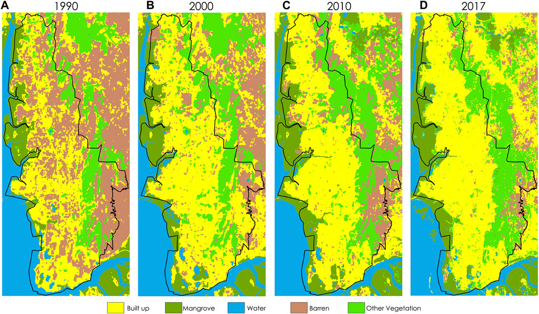
Figure 6. Land cover map of Navi Mumbai city created with Landsat data for the years (A) 1990, (B) 2000, (C) 2010 and (D) 2017.

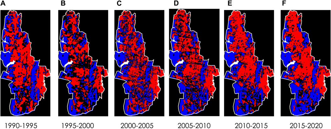
Figure 7. Thermal conditions of pixels identified from the spatial LST anomaly over Navi Mumbai. Each sub-plot from (A–F) indicates a 5-year block starting from 1990. Colour coding is the same as Figure 4.

To understand the spatial pattern of the spatial LST anomaly (${\text{LST}}_{\text{ano}}^{\mathrm{S}}$), SUHII maps have been developed for both cities. Figure 8 shows the SUHII observed Navi Mumbai municipal corporation area and it can be observed that the city has become progressively warmer with hot spots located in bare surfaces and core residential areas of the city. Hot spots were also observed in between the green cover of Mangroves present in the city, indicating the change in land cover over the years. Towards the southeastern part of the city, lies Parsik hill (marked as a red patch in the southeastern part of the city in Figure 8) which experiences warmer conditions compared to other vegetated areas in the city due to the sparse vegetation conditions, construction and quarrying activities carried out in this region over a long period of time. In Navi Mumbai, the cooling effect of mangroves and water bodies along the city boundaries was evident. This observation is consistent with the findings of Keith and Meerow (2022), who highlighted the role of coastal vegetation in mitigating urban heat. The spatial anomaly maps also revealed that core urban areas with densely developed surfaces showed higher LST anomalies, corroborating studies that associate high impervious surface coverage with increased UHI intensity (Santamouris, 2015).

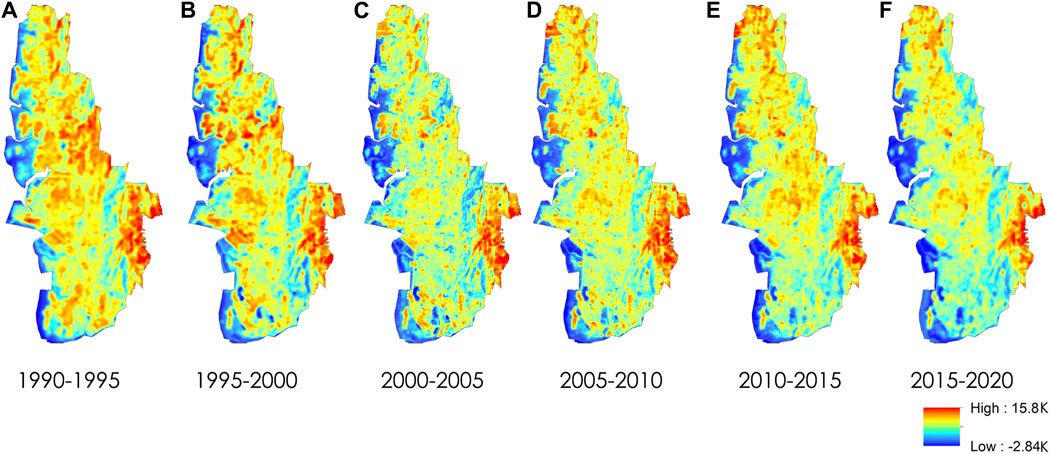
Figure 8. SUHII evolution over Navi Mumbai. (A) 1990–1995, (B) 1995–2000, (C) 2000–2005, (D) 2005–2010, (E) 2010–2015, (F) 2015–2020.

Figures 9, 10 show the change in spatial LST anomaly and SUHII, respectively during different time periods over the Chennai Metropolitan area (CMA). Several areas that have been classified as warm pixels in Figure 9 can be seen to have positive SUHII values in Figure 10. For example, the crescent-shaped green patch in the centre of the area marked “i” in Figure 10 indicates a water body. Over the years, there has been a shrinkage in the size of this water body, causing the area surrounding the water body to become warmer. Similarly, the airport area, marked as “ii”, also shows warming conditions. It can be seen that the area has become warmer with the development of the secondary runway and taxiways over the years. On the other hand, the area marked “iii” appears cooler compared to the other parts of the city. The location corresponds to the estuary of the Adyar river, which flows through Chennai. This area is a mix of vegetation, water bodies and well-developed built-up areas with multiple high-rise structures. The proximity of the sea with its cool sea breezes, the channelling of the wind by the tall well developed buildings and the presence of vegetation in the surroundings play a major role in lowering the temperature in this area. The spatial analysis revealed the cooling buffer zones created by the natural cover, including vegetation and water bodies, located in close proximity to the developed spaces. The spatial anomaly analysis highlighted that water bodies and vegetated areas consistently exhibited negative anomalies, indicating cooler conditions. This finding is supported by the literature, which emphasises the cooling effects of vegetation and water bodies in urban environments. For example, Bowler et al. (2010) noted that urban green spaces can reduce local temperatures by up to 1.5°C, while Wu et al. (2019) reported that water bodies contribute to cooling through evapotranspiration. The spatial anomaly value for vegetation and water ranged from −2.5 to 0, indicating significant cooling potential, while built spaces located in proximity to natural cover exhibited a value ranging from −0.5 to 0.5, highlighting the role of natural infrastructure in mitigating the UHI effect.

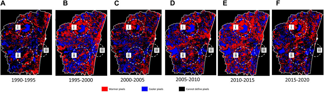
Figure 9. Thermal conditions of pixels identified from spatial LST anomaly over Chennai Metropolitan Area. Each sub-plot from (A–F) indicates a 5-year block starting from 1990. Colour coding is the same as Figure 4.

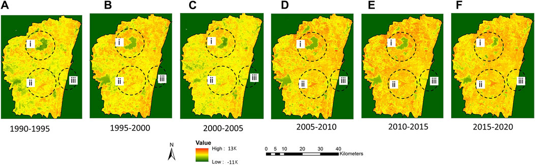
Figure 10. SUHII evolution over Chennai. (A) 1990–1995, (B) 1995–2000, (C) 2000–2005, (D) 2005–2010, (E) 2010–2015, (F) 2015–2020.

Our results indicate that planned settlements developed on barren land with vegetation cover and near water bodies with proper street and building orientation have temporal anomaly values similar to those of vegetated surfaces, ranging from 0.08 to 1. This finding underscores the importance of site-level urban design in mitigating the large-scale UHI effect and the microclimate of the region. Studies by Norton et al. (2015) and Emmanuel and Krüger (2012) support this finding, highlighting that strategic urban planning and design, including green infrastructure and optimal street orientation, can significantly reduce urban temperatures.

Further Assessment of LST Anomalies

Assessment of LST Anomaly Classification

The pixels labelled as warm and cool on the spatial LST anomaly maps and temporal LST anomaly maps were subjected to further assessment by visual examination. High resolution images available on Google Earth were used to compare the land cover state of the area with the classification on the LST anomaly maps. Over surfaces that changed from a natural state to other states (such as impervious urban surfaces), the LST anomaly exhibited a clear change in sign and magnitude from negative to positive and remained positive for most of the years after the change occurred. The reverse was also noted, for example, over Navi Mumbai, the growth of vegetation over barren surfaces resulted in the areas becoming cooler and hence, exhibiting negative LST anomalies. A few examples have been added in the online Supplementary Material to support the findings (Supplementary Figures S2–S4).

From each anomaly change map (presented in Figures 3, 4, 7, 9), points labelled as warm and cool were randomly selected and compared with high resolution images available on Google Earth obtained in the corresponding time period. In the high-resolution visual images available on Google Earth corresponding to the 5-year window of the anomaly change maps, the land cover of the particular location was noted. If the land cover of the particular location was either barren or built up for the majority of the time in the 5-year window, then it was considered a warm pixel. Similarly, if the land cover was a vegetated area or water body, then the location was labelled as a cool pixel. Thus, if a pixel was labelled as warm in the anomaly change maps, it should correspond to barren or developed to be tagged as correctly classified. Similarly, a cool pixel was assumed to be correctly classified if it corresponded to a vegetated surface or water body. With this interpretation, the accuracy of both spatial and temporal anomaly change maps, was evaluated and the results are presented in Table 1. This is an indirect evaluation of the thermal anomaly change maps as no reference data were available for making a direct comparison with the LST anomaly maps, as is usually done for a land cover map.

Table 1. Results of visual evaluation of LST anomaly change maps.

From Table 1, it can be observed that the anomaly change maps consistently corresponded to warm or cool pixels for more than 80% of the pixels tested and for both cities. This suggests that the anomaly change map can act as an indicator of surfaces that have become impervious from their natural state and vice versa. The accuracy assessment method presented here will erroneously classify all developed spaces as warmer places. As mentioned, a few developed areas adjacent to water bodies in both Chennai and Navi Mumbai have become cooler over time. However, such places are rather limited and as an overall pattern, barren surfaces and developed areas exhibited warmer temperatures compared to vegetated surfaces.

Comparison Between Navi Mumbai and Chennai

Although the aim of this study is to demonstrate the potential of LST anomalies in identifying changes in the thermal regime of cities, the analysis of two study areas offered an opportunity to compare the two cities. Table 2 presents the percentage of pixels (with respect to the total number of pixels in the city) with a given temporal LST anomaly value (rounded off to an integer) for Chennai and Navi Mumbai for the years 1989 1990 and 2020. Observing the values in Table 2, it can be inferred that both cities have warmed up significantly compared to the past. LST values are increasing over both cities with time leading to this warming trend. In particular, Chennai which had almost 100% of the pixels equal to or less than the long-term LST mean in 1990 now has more than 43% of the pixels greater than the long-term LST mean. There is also a considerable decrease in the number of pixels exhibiting negative anomalies. Navi Mumbai has also warmed significantly with a notable increase in the number of pixels with positive LST anomalies in 2020. However, unlike Chennai, Navi Mumbai also had LST hot spots in the past indicated by the presence of approximately 44% of pixels with positive temporal LST anomalies. In terms of LST, Chennai was relatively cooler in the past than in the present.

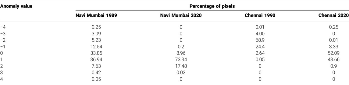
Table 2. Percentage of pixels with different temporal LST anomaly values in Chennai and Navi Mumbai.

Table 3 presents a similar analysis, but with spatial anomalies. It should be recalled that the spatial LST anomaly indicates the relative temperature difference of a pixel with respect to the mean LST in the city. In the Table 3, it can be observed that the overall pattern of spatial LST anomalies over Navi Mumbai remained more or less similar in 2020 compared to 1989. This is also evident from the SUHII images for Navi Mumbai shown in Figure 8. Navi Mumbai had open and hot barren surfaces in 1990 which were converted to developed areas in the following years (Figure 6). This could be the reason for the similar spatial LST anomaly patterns. Chennai, on the other hand, has become warmer with a decrease in the number of pixels with negative LST anomalies and an increase in the number of pixels with positive spatial anomalies. This can also be observed in the SUHII maps for Chennai (Figure 10). These results indicate that the city of Chennai is becoming warmer with time and many pixels are becoming hot spots.

Table 3. Percentage of pixels with different spatial LST anomaly values in Chennai and Navi Mumbai.

Conclusion

There is a transition from natural land cover (vegetation/water) to barren and impervious land cover during urbanisation. From an urban planning perspective, it is imperative to understand the change in thermal conditions of a city due to urbanisation and provide solutions to mitigate the resulting heat effect. This study utilised thermal anomalies to identify changes in land cover conditions over urban areas that can be related to urban growth over the years. This study highlighted the hotspot areas in an urban settlement indicating the zones where quick action is required in developing effective strategies to mitigate the impact of urbanisation on SUHII and improve the liveability of the cities. The results of this study can also be utilised to develop area specific policies for a sustainable habitat. They also open up a space to study how planned settlements behave thermally over the years. Finally, they highlight the need to plan cities that are adaptable and resilient to urban heat due to development pressure.

In this study, the temporal anomaly maps were developed using data over a period of 32 years (1988–2020). LST values could have increased naturally over the two cities and this could have caused a large part of the cities to appear warm compared to the early 1990s (Figures 3F, 4F). Although the long-term mean has been used here, a relatively shorter time period (10 or 15 years) can be used especially for cities that have recently developed.

The present work was limited to summertime anomalies as they show clearer results compared to the winter season anomalies. This study can be further developed by comparing the results from nighttime LST data to see the shift in SUHII over day and night. However, high resolution LST data from Landsat-like satellites are not available at night. Furthermore, using LST from MODIS at 1 km may not capture the finer-scale LST variations. Recent and upcoming thermal sensors such as ECOSTRESS, TRISHNA, LSTM and SBG can provide relatively finer resolution LST even at night and these can be utilised for the analysis. In addition, for analysing the datasets in the past, thermal disaggregation methods developed in studies such as Sara et al. (2024) can be utilised to disaggregate MODIS LST to a finer spatiotemporal scale for LST analysis.

Data Availability Statement

The Landsat images used in the study are publicly available in the Google Earth Engine platform. Further inquires, if any can be directed to the corresponding author.

Author Contributions

Conceptualization, methodology, data collection, analysis, writing: ER and AR. Thermal data analysis: RH. Land cover mapping and analysis: LG. All authors contributed to the article and approved the submitted version.

Funding

The authors declare that no financial support was received for the research, authorship, and/or publication of this article.

Conflict of Interest

The authors declare that the research was conducted in the absence of any commercial or financial relationships that could be construed as a potential conflict of interest.

Publisher’s Note

All claims expressed in this article are solely those of the authors and do not necessarily represent those of their affiliated organizations, or those of the publisher, the editors and the reviewers. Any product that may be evaluated in this article, or claim that may be made by its manufacturer, is not guaranteed or endorsed by the publisher.

Supplementary Material

The Supplementary Material for this article can be found online at: https://www.escubed.org/articles/10.3389/esss.2024.10096/full#supplementary-material

References

Azeez, S. A., Gnanappazham, L., Muraleedharan, K., Revichandran, C., John, S., Seena, G., et al. (2022). Multi-Decadal Changes of Mangrove Forest and Its Response to the Tidal Dynamics of Thane Creek, Mumbai. J. Sea Res., 1–14. doi:10.1016/j.seares.2021.102162
Bechtel, B., Demuzere, M., Mills, G., Zhan, W., Sismanidis, P., Small, C., et al. (2019). SUHI Analysis Using Local Climate Zones—A Comparison of 50 Cities. Urban Clim. 28, 100451. doi:10.1016/j.uclim.2019.01.005
Bowler, D. E., Buyung-Ali, L., Knight, T. M., and Pullin, A. S. (2010). Urban Greening to Cool Towns and Cities: A Systematic Review of the Empirical Evidence. Landsc. Urban Plan. 97 (3), 147–155. doi:10.1016/j.landurbplan.2010.05.006
Chen, Y., Yang, J., Yu, W., Ren, J., Xiao, X., and Xia, J. C. (2023). Relationship Between Urban Spatial Form and Seasonal Land Surface Temperature Under Different Grid Scales. Sustain. Cities Soc. 89, 104374. doi:10.1016/j.scs.2022.104374
Deilami, K., Kamruzzaman, M., and Liu, Y. (2018). Urban Heat Island Effect: A Systematic Review of Spatio-Temporal Factors, Data, Methods, and Mitigation Measures. Int. J. Appl. Earth Observation Geoinformation 67, 30–42. doi:10.1016/j.jag.2017.12.009
Dousset, B., and Luvall, J. C. (2019). “Surface Temperatures in the Urban Environment,” in Taking the Temperature of the Earth: Steps Towards Integrated Understanding of Variability and Change. Editor G. C. Hulley (Elsevier Science), 203–226. doi:10.1016/B978-0-12-814458-9.00007-1
Emmanuel, R., and Krüger, E. (2012). Urban Heat Island and Its Impact on Climate Change Resilience in a Shrinking City: The Case of Glasgow, UK. Build. Environ. 53, 137–149. doi:10.1016/j.buildenv.2012.01.020
Ermida, S. L., Soares, P., Mantas, V., Göttsche, F. M., and Trigo, I. F. (2020). Google Earth Engine Open-Source Code for Land Surface Temperature Estimation From the Landsat Series. Remote Sens. 12 (9), 1471. doi:10.3390/RS12091471
Geletič, J., Lehnert, M., Savić, S., and Milošević, D. (2019). Inter-/Intra-Zonal Seasonal Variability of the Surface Urban Heat Island Based on Local Climate Zones in Three Central European Cities. Build. Environ. 156, 21–32. doi:10.1016/j.buildenv.2019.04.011
Grumm, R., and Hart, R. (2001). Standardized Anomalies Applied to Significant Cold Season Weather Events: Preliminary Findings. Weather and Forecast. 16 (6), 736–754. doi:10.1175/1520-0434(2001)016<0736:SAATSC>2.0.CO;2
Han, D., An, H., Wang, F., Xu, X., Qiao, Z., Wang, M., et al. (2022). Understanding Seasonal Contributions of Urban Morphology to Thermal Environment Based on Boosted Regression Tree Approach. Build. Environ. 226, 109770. doi:10.1016/j.buildenv.2022.109770
Harod, R., Rajasekaran, E., and Bhattacharya, B. K. (2021). Effect of Surface Emissivity and Retrieval Algorithms on the Accuracy of Land Surface Temperature Retrieved From Landsat Data. Remote Sens. Lett. 12 (10), 983–993. doi:10.1080/2150704X.2021.1957511
IPCC (2021). Climate Change 2021: The Physical Science Basis. Contribution of Working Group I to the Sixth Assessment Report of the Intergovernmental Panel on Climate Change.
Julien, Y., and Sobrino, J. A. (2008). The Yearly Land Cover Dynamics (YLCD) Method: An Analysis of Global Vegetation From NDVI and LST Parameters. Remote Sens. Environ. 113 (2), 329–334. doi:10.1016/j.rse.2008.09.016
Keith, L., and Meerow, S. (2022). Planning for Urban Heat Resilience. Chicago: American Planning Association.
Keith, L., Meerow, S., and Wagner, T. (2019). Planning for Extreme Heat: A Review. J. Extreme Events 06 (3 & 4), 2050003–2050027. doi:10.1142/s2345737620500037
Kodimalar, T., Vidhya, R., and Rajasekaran, E. (2020). Land Surface Emissivity Retrieval From Multiple Vegetation Indices: A Comparative Study Over India. Remote Sens. Lett. 11 (2), 176–185. doi:10.1080/2150704X.2019.1692384
Li, D., Liao, W., Rigden, A. J., Liu, X., Wang, D., Malyshev, S., et al. (2019). Urban Heat Island: Aerodynamics or Imperviousness? Sci. Adv. 5 (4), eaau4299. doi:10.1126/sciadv.aau4299
Li, X., Zhou, Y., Asrar, G. R., Imhoff, M., and Li, X. (2017). The Surface Urban Heat Island Response to Urban Expansion: A Panel Analysis for the Conterminous United States. Sci. Total Environ. 605-606, 426–435. doi:10.1016/j.scitotenv.2017.06.229
Martilli, A., Krayenhoff, E. S., and Nazarian, N. (2020). Is the Urban Heat Island Intensity Relevant for Heat Mitigation Studies? Urban Clim. 31, 100541. doi:10.1016/j.uclim.2019.100541
Mildrexler, D. J., Cohen, W. B., Zhao, M., Running, S. W., Song, X.-P., and Jones, M. O. (2018). Thermal Anomalies Detect Critical Global Land Surface Changes. J. Appl. Meteorology Climatol. 57 (2), 391–411. doi:10.1175/JAMC-D-17-0093.1
Mildrexler, D. J., Zhao, M., and Running, S. W. (2009). Testing a MODIS Global Disturbance Index Across North America. Remote Sens. Environ. 113 (10), 2103–2117. doi:10.1016/j.rse.2009.05.016
Muro, J., Strauch, A., Heinemann, S., Steinbach, S., Thonfeld, F., Waske, B., et al. (2018). Land Surface Temperature Trends as Indicator of Land Use Changes in Wetlands. Int. J. Appl. Earth Observation Geoinformation 70, 62–71. doi:10.1016/j.jag.2018.02.002
Norton, B. A., Coutts, A. M., Livesley, S. J., Harris, R. J., Hunter, A. M., and Williams, N. S. (2015). Planning for Cooler Cities: A Framework to Prioritise Green Infrastructure to Mitigate High Temperatures in Urban Landscapes. Landsc. Urban Plan. 134, 127–138. doi:10.1016/j.landurbplan.2014.10.018
Santamouris, M. (2015). Analyzing the Heat Island Magnitude and Characteristics in One Hundred Asian and Australian Cities and Regions. Sci. Total Environ. 512-513, 582–598. doi:10.1016/j.scitotenv.2015.01.060
Sara, K., Rajasekaran, E., Nigam, R., Bhattacharya, B. K., Kustas, W. P., Alfieri, J. G., et al. (2024). Combining Spatial Downscaling Techniques and Diurnal Temperature Cycle Modelling to Estimate Diurnal Patterns of Land Surface Temperature at Field Scale. PFG. doi:10.1007/s41064-024-00291-1
Shastri, S. H., and Ghosh, S. (2019). “Urbanisation and Surface Urban Heat Island Intensity (SUHII),” in Climate Change Signals and Response (Singapore: Springer), 73–90. doi:10.1007/978-981-13-0280-0_5
Sobrino, J. A., and Raissouni, N. (2010). Toward Remote Sensing Methods for Land Cover Dynamic Monitoring: Application to Morocco. Int. J. Remote Sens. 21 (2), 353–366. doi:10.1080/014311600210876
Stewart, I. D., and Oke, T. R. (2012). Local Climate Zones for Urban Temperature Studies. Bull. Am. Meteorological Soc. 93 (12), 1879–1900. doi:10.1175/BAMS-D-11-00019.1
Stewart, J. D., and Kremer, P. (2022). Temporal Change in Relationships Between Urban Structure and Surface Temperature. Environ. Plan. B Urban Anal. City Sci. 49 (9), 2297–2311. doi:10.1177/23998083221083677
Wu, C., Li, J., Wang, C., Song, C., Chen, Y., Finka, M., et al. (2019). Understanding the relationship between urban blue infrastructure and land surface temperature. Sci. Total Environ. 694, 133742. doi:10.1016/j.scitotenv.2019.133742
Yuan, F., and Bauer, M. E. (2006). Comparison of Impervious Surface Area and Normalized Difference Vegetation Index as Indicators of Surface Urban Heat Island Effects in Landsat Imagery. Remote Sens. Environ. 106 (3), 375–386. doi:10.1016/j.rse.2006.09.003
Zhao, L., Lee, X., Smith, R. B., and Oleson, K. (2014). Strong Contributions of Local Background Climate to Urban Heat Islands. Nature 511 (7508), 216–219. doi:10.1038/nature13462
Zhao, Z. Q., He, B. J., Li, L. G., Wang, H. B., and Darko, A. (2017). Profile and Concentric Zonal Analysis of Relationships Between Land Use/Land Cover and Land Surface Temperature: Case Study of Shenyang, China. Energy Build. 155, 282–295. doi:10.1016/j.enbuild.2017.09.046
Zhou, D., Xiao, J., Bonafoni, S., Berger, C., Deilami, K., Zhou, Y., et al. (2018). Satellite Remote Sensing of Surface Urban Heat Islands: Progress, Challenges, and Perspectives. Remote Sens. 11 (48), 48–36. doi:10.3390/rs11010048
Keywords: Land Surface Temperature anomaly, surface urban heat island, landcover change, remote sensing, green infrastructure
Citation: Roy A, Rajasekaran E, Harod R and Gnanappazham L (2024) Land Surface Temperature Anomalies as Indicators of Urban Land Cover Change—A Study of Two Indian Cities. Earth Sci. Syst. Soc. 4:10096. doi: 10.3389/esss.2024.10096
Received: 24 September 2023; Accepted: 05 August 2024;
Published: 20 August 2024.
Edited by:
Bakul Budhiraja, Queen’s University Belfast, United KingdomReviewed by:
Yusuf Aina, Royal Commission for Jubail and Yanbu, Saudi ArabiaAdinarayanane Ramamurthy, School of Planning and Architecture Vijayawada, India
Copyright © 2024 Roy, Rajasekaran, Harod and Gnanappazham. This is an open-access article distributed under the terms of the Creative Commons Attribution License (CC BY). The use, distribution or reproduction in other forums is permitted, provided the original author(s) and the copyright owner(s) are credited and that the original publication in this journal is cited, in accordance with accepted academic practice. No use, distribution or reproduction is permitted which does not comply with these terms.
*Correspondence: Eswar Rajasekaran, ZXN3YXIuckBjaXZpbC5paXRiLmFjLmlu